Posted by Osvaldo
July 7, 2016
If all tests are negative, the positive rate is zero. And its confidence interval?
Some time ago a colleague presented me a simple statistics question which, as usual, turned out to be quite interesting and intriguing. They had run 23 tests that were all negative, and they wanted to have a confidence interval for the proportion of positive outcomes. So, to put it in statistical terms, we have \(n\) observations that can be \(0\) or \(1\). Each observation has a probability \(\theta\) of being positive. In formulas
\[ x_i \in \{0, 1\} \quad \forall i = 1, \ldots , n \\ p(x_i=1) = \theta . \]
We know that the number of successes is binomially distributed, thus a sufficient statistics is \(T = \sum_i x_i\) and that the maximum likelihood estimator for the binomial proportion is
\[ \hat{\theta} = \frac{T}{n} . \]
If the observations are all negative, the estimate for the rate is clearly zero, but what about its confidence interval? I had never been asked to estimate the confidence interval for the binomial distribution, so I was totally unprepared (shame on me!). Quite instinctively, I computed the probability to observe all 23 results negative for a given \(\theta\), set this to 5% and solved for \(\theta\). Result, 12.2%. In formula
\[ p(\mathrm{all\;negatives}\, |\, \theta) = (1-\theta)^n \leq \alpha, \]
which gives, solving for \(\theta\),
\[ \theta_u = 1 - \alpha^{1/n} \\ \theta_u(n=23) = 12.2\% . \]
In other words, what I did was to compute the highest \(\theta\) for which I would be very surprised (5%) to see all negative outcomes. This is equivalent to being quite sure (95% sure) to observe at least one positive outcome.
My colleague had found the formula for the Clopper-Pearson interval and applied it to their case: different result. Of course, I thought: I computed the probability to observe data as extreme or more extreme than those observed for a given value of the parameter. I did a hypothesis test, not a confidence interval.
It would have been the end of the story, had I not tried this online calculator. It reports \(0 \leq \theta \leq 0.12\) to be the 90% interval for \(n=23\). This was no coincidence, as the plot below shows.
In other words, for any number of tests (at least, between five and thirty) my estimate (violet points) matches the upper limit of the 90% confidence interval computed with the Clopper-Pearson method (magenta line).
library(ggplot2)
library(ggthemr)
ggthemr('solarized', type='outer')

# computing 90% confidence interval with "exact" meaning Clopper-Pearson
library(binom)
cis <- binom.confint(0, 5:30, conf.level = 0.9, methods="exact")

# max theta for which n all negative outcomes have probability 5%
p_all_neg <- 1-0.05**(1./5:30)

df <- data.frame(x=5:30, y1=cis$upper, y2=p_all_neg)
p <- ggplot(df, aes(x)) +
  geom_line(y = df$y1, show.legend = TRUE, colour='#d33682') +
  geom_point(y = df$y2, show.legend = TRUE, colour='#6c71c4') +
  xlab("trials") +
  ylab(expression(theta)) +
  ylim(0.0, 0.5) +
  theme(axis.title.x = element_text(face="bold", size=18),
        axis.text.x  = element_text(angle=0, vjust=0.0, size=14),
        axis.title.y = element_text(face="bold", size=18),
        axis.text.y  = element_text(angle=0, vjust=0.0, size=14))
print(p)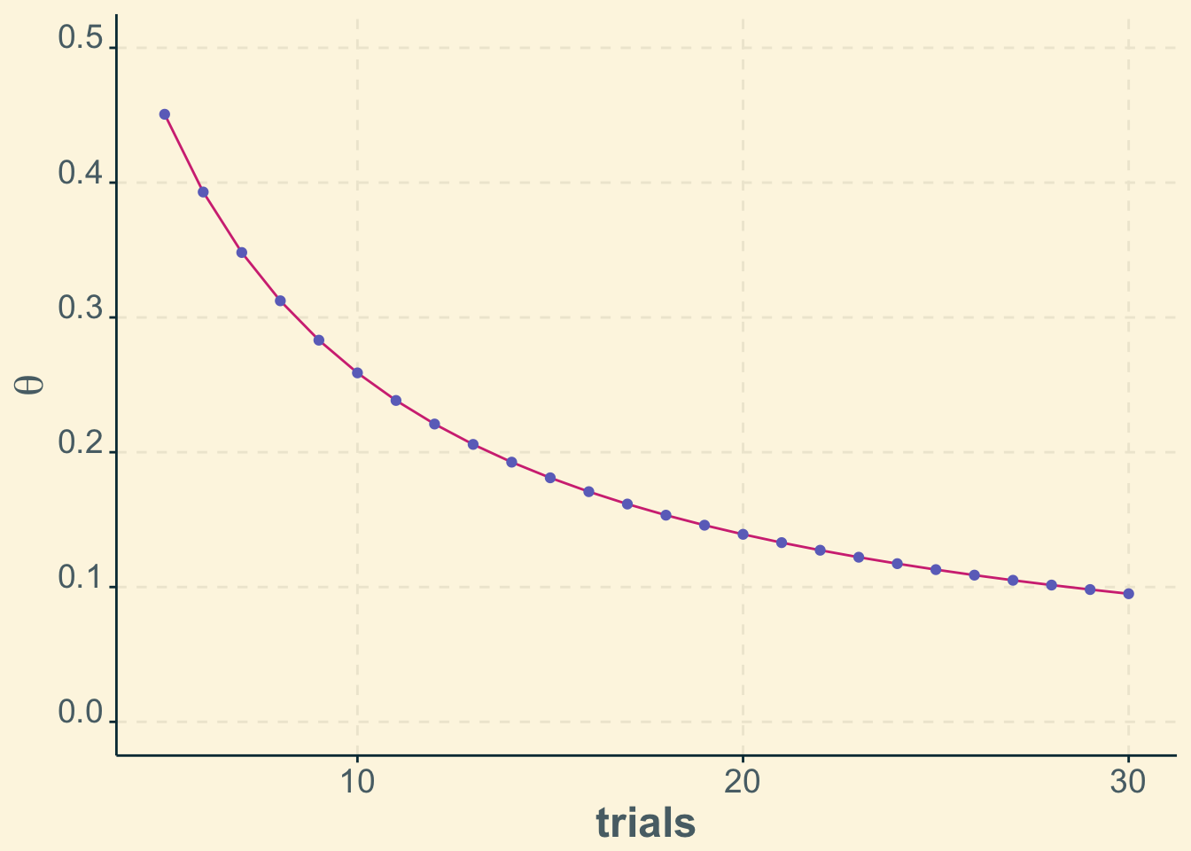
Finding confidence intervals
There is a one-to-one correspondence between confidence intervals and hypothesis tests. As a matter of fact, confidence sets are found by inverting a test statistics.
Let’s start revisiting a few concepts, following the classics. We have a hypothesis for a parameter of interest \(\theta\). The hypothesis says that it has a certain value
\[ H_0 : \theta = \theta_0. \]
We have data \(X\) and a test statistics telling us whether to reject the hypothesis or not. The acceptance region \(A(\theta_0)\) is the region of the sample space for which we do not reject \(H_0\) at a level \(\alpha\). In symbols
\[ p(X \in A(\theta_0)) \geq 1 - \alpha \]
or
\[ p(X \notin A(\theta_0)) \leq \alpha. \]
Now, for each realisation of the data \(X\), we take the values of \(\theta\) for which the hypothesis \(H_0\) is accepted. Then we have built a confidence set for \(\theta\). We define \(C(X)\) as the set in parameter
\[ C(X)=\{\theta_0 : x \in A(\theta_0)\}. \]
Then, \(C(X)\) is a \(1 - \alpha\) confidence set. This follows quite immediately from the definition of acceptance region above
\[ p(\theta \in C(X)) = p(X \in A(\theta_0)) \geq 1 − \alpha. \]
Clopper-Pearson estimator
There are several estimators for the confidence interval of the binomial proportion. The advantage of this one is that it is exact, rather than based on the normal approximation (see the Wikipedia page linked above). The disadvantage is that it is conservative, i.e. there might be a smaller interval with the same confidence level. The estimated interval is defined as
\[ \{\theta : p(\mathrm{Bin}(n, \theta) \leq T) > \frac{\alpha}{2} \} \cap \{\theta : p(\mathrm{Bin}(n, \theta) \geq T) > \frac{\alpha}{2} \}. \]
From this definition we reconcile the fact that my estimate at 95% coincides with the Clopper-Pearson at 90%. In fact, since we are in the special case of \(T=0\), we can write the Clopper-Pearson as
\[ \{\theta : p(\mathrm{Bin}(n, \theta) \leq 0) > \frac{\alpha}{2} \} \cap \{\theta : p(\mathrm{Bin}(n, \theta) \geq 0) > \frac{\alpha}{2} \} = \{\theta : p(\mathrm{Bin}(n, \theta) = 0) > \frac{\alpha}{2} \}. \]
By taking \(\alpha = 0.10\) in the Clopper-Pearson estimate, we have the formula I used for my estimate.
A final observation
What is most interesting to my colleague? The hypothesis test says that those data would already exclude \(\theta=0.12\) or higher at 5%, but the 95% interval according to Clopper-Pearson is \(0 \leq \theta \leq 0.15\). As we saw they are two different but intimately related things. What is more important to you depends largely on your taste. We also had the chance to underline something that is often neglected: finding an \(\alpha\) confidence interval doesn’t mean we found the smallest interval that contains the true value with probability \(1 - \alpha\). If you want to investigate an extreme consequence of this, you can visit the ultimate confidence intervals calculator.
Header image from Flickr