Posted by Osvaldo
November 20, 2016
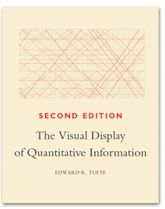
If you look at the front cover of The Visual Display of Quantitative Information, one of the famous books by Eduard Tufte, you will see a plot made of many lines. An intricate network of red lines of different thickness, cutting diagonally a regular grey grid.
The plot is one of the examples of the first chapter, Graphical Excellence, and it is a graphical train schedule for Paris to Lyon in 1880s, by Étienne-Jules Marey. The station are arranged vertically (the top one being Paris) at a distance proportional to their actual distance, while time is on the horizontal axis. Each line is a train, and the slope is the speed. It took around nine hours for the entire trip but the TGV, first introduced in 1981, completes the trip in less than three hours. A red line overlayed on the schedule of 100 years before marks the progress made.
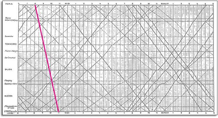
I like these plots because of their simplicity: position vs. time; something I must have seen for the first time in secondary school or even earlier. Angle, slope, tangent, derivative, speed, everything is there, you just name it differently in different moments of your education.
I decided to reproduce this plot for the Zurich-Milano train connection, which is about to experience an historical moment. In a few weeks, all passenger trains on this line will be traveling in the Gotthard Base Tunnel. It is the world’s longest tunnel, running along more than 57 km under the Swiss Alps at an altitude between 469 and 312 m. Trains currently travel through another tunnel, the Gotthard Tunnel, 15 km long, built at the end of 19th century at an altitude of around 1,100 m. In order to climb to that altitude, trains travel through several railway spirals. The view is great, but the speed is not.
I downloaded the schedule for a few morning trains that go through the Panoramastrecke (the panoramic track) and a few that will go through the base tunnel, they are shown in the plot below. It might not look that impressive compared to the TGV. But if you look at the mountains while approaching them from the plain, it’s a different feeling.

Nine people died during construction of the Gotthard Base Tunnel. None of them was of Swiss nationality.
Below is the R code used to produce the schedule plot. The timetable for a few train was obtained on the SBB website and manually written into a csv file. The coordinates of the cities were taken on Google Maps and saved here.
library(tidyverse)
library(ggthemr)
ggthemr('solarized', type='outer')
library(geosphere)

# parse coordinates and compute distances
coordinates_table <-
  read_csv("train_gotthard/coordinates-table.csv")
cities <- coordinates_table$city
coordinates_table$city <- NULL
p1 <- as.matrix(coordinates_table)
p2 <- matrix(c(rep(p1[1, 1], length(cities)), rep(p1[1, 2], length(cities))), ncol=2)
dists <- distHaversine(p1, p2)

trains <-
  read_csv("train_gotthard/timetable-table.csv",
          col_types = cols(city = col_character(),
                           time = col_character(),
                           train = col_character(),
                           track = col_character())) %>%
  mutate(time=as.POSIXct(time, format="%H:%M"))
distances <- data_frame(city=cities, d=dists)

trains <- trains %>%
  full_join(distances, by="city") %>%
  mutate(train_track=paste(train, track, sep='_'))

cbPalette <- c("#657b83", "#268bd2")
p <- ggplot(trains, aes(x=time, y=d, group=train_track, colour=track)) +
  geom_line() +
  scale_y_continuous(breaks=distances$d, labels=distances$city) +
  scale_x_datetime(date_breaks = "1 hour", date_labels = "%H:%M") +
  xlab('') + ylab('') +
  theme(axis.title.x = element_text(size=15),
        axis.text.x  = element_text(size=15),
        axis.title.y = element_text(size=15),
        axis.text.y  = element_text(size=15),
        legend.title = element_text(size=15),
        legend.text  = element_text(size=15)) +
  scale_colour_manual(values=cbPalette)
Header image via Flickr (under CC BY-ND 2.0).